Second growth:The promise of tropical forest regeneration in an age of deforestation

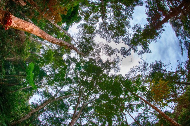
IMG_20160113_112417

Anyone who knows anything about secondary forests will have come across the work of Robin Chazdon. She has inspired at least one forest ecologist, me, that forests recovering from major disturbances are a subject worthy of study. I’m sure she has done the same for many others out there. So, coming towards the end of my PhD I was excited to see a book that she had written summarising the topic was due to be released and using the last of my NERC funds I bought it. And then I moved house to Spain, where the book sat untouched and unloved in a box for the next year. After I came back to the UK last year, I found the book again and decided I should stop putting off reading it. I read it on trains, buses, on my sofa and occasionally in bed. I once fell asleep reading this book, though admittedly that was on the way back from the BES annual meeting  in Edinburgh, and the gin from the previous night was probably the cause of my sleepiness rather than any bad writing.

The first thing to say is that this book is extremely comprehensive. Though it is not particularly lengthy, running to 316 pages of text, it covers a huge range of topics relating to forest regeneration from traditional knowledge and prehistoric forest transformations by humans to recovery pathways from fire, landslides, volcanic eruptions, logging, and agricultural use. There are also numerous sections on community assembly, functional traits, ecosystem function, and animal and plant interactions. The last section concentrates on reforestation and restoration of degraded forests, making a passionate plea for degraded forests to not be considered as wasteland.

For me the most fascinating parts of the book were those that covered traditional knowledge of forest regeneration and the history of human cultures in tropical forests – both subjects I knew practically nothing about before this book. I was captivated to read that the dayak people of Borneo have five words to define different stages of forest recovery – kurat uraq (1-3 year old scrub that forms after abandonment), kurat tuha (trees > 5 cm in diameter and 5-6 metres in height), kurat batang muda (trees 10-15 cm in diameter), kurat batang tuha (closed canopy secondary forest) and hutan bengkar (primary forest). As Chazdon points out this knowledge shows a striking resemblance to that of forest ecologists. Similarly, Mayan cultures in Central America and Soliga people in the Western Ghats have developed a subtle knowledge of the stages of forest succession. I have always been a bit skeptical of integrating traditional knowledge into ecological science, but this book convinced me that there could be some value to it.

Chazdon masterfully weaves together anthropology, archaeology and ecology in the discussion of prehistorical impacts of humans on tropical forests. She cites evidence of earthworks called geoglyphs similar to the Nazca lines found in the state of Acre in Brazil, swidden agriculture 20,000 years ago in Papua New Guinea and human populations in Central America to dispel the view that any forest is truly untouched. There are probably legacies of human use in most forests, we just can’t identify them. Based on this she, perhaps controversially, critiques recent work suggesting that mature tropical forest biomass density is increasing as a result of atmospheric carbon dioxide. Chazdon’s view is that this increase could well be as a result of recovery from unseen disturbances that happened generations ago.

The section on community turnover during succession is also excellent, with a detailed analysis of the characteristics of short- and long-lived pioneer and shade tolerant, late successional species. At points Chazdon playfully conjures up text resembling Shakespeare’s  “All the world’s a stage” monologue: “The term successional stage is apt. Successional pathways can be viewed as an improvisational drama in several acts, with each act featuring a different set of actors. Some actors perform throughout the drama, but others have cameo appearances of only one act. Although each act sets the stage for the next, forest regeneration has no director and only a roughly sketched script creating a high degree of spontaneity, randomness and uncertainty.” These are amongst my favourite parts of the book, with metaphor mixing with a solid science to help things stick in your mind that might otherwise be easily forgotten.

If I have any criticism of the book, it is that it’s a bit repetitive. This is probably because Chazdon sees succession as ‘an improvisational drama in several acts’ and so the book relies on case studies, rather than synthesising current knowledge to form generalities. However, I think that the repetition helps if you just want to dip in and out of chapters – I don’t think it is necessarily written to be read cover to cover like I did.

That aside if you are interested in the dynamics of forests in any way this book is essential reading. There is no better summary of current thinking on tropical forest succession out there.

Is ecological succession predictable?

Over the last few years I have written quite a lot about forest succession. I have published a paper on the topic, have a paper in review about recovery of a forest under multiple stressors and will be starting more work on the it over the next few weeks. All in all, I think I have a reasonable idea what I’m talking about when it comes to succession, at least in forests. However, I’ve just read a paper on tropical forest succession that caught me a bit unawares*.

The paper in question is Natalia Norden and colleagues’ work that was recently published in PNAS. The authors collected data from 72 secondary forest plots monitored for 7-24 years at 7 different sites across tropical South and Central America. They then used this data to look whether we can predict trajectories plot stem density, basal area and species density during forest succession after total clearance. On the whole the paper found that trajectories were poorly predicted by models that looked at change as a function of forest age. From the figure below, you can pick some general trends in the direction of change with age – stem density might have a humped relationship with age for example. However, it is also clear that there is a huge amount of variation and some trajectories bounce around all over the place.

Observed successional trajectories of stem density, basal area and species density for the sites used by Norden et al.

It’s obvious from looking at the figure above that the age of a secondary forest doesn’t really act as a proxy for its successional stage. In fact Norden and colleagues found that on average age only explains 20% of within site variation. Even if that is better than the average ecology paper, it’s still not very good. To explain the rates of change of different variables, Norden et al. fitted a set of different non-linear models for each site. Again, their findings emphasised the large amount of variation between different sites. Due to these idiosyncrasies, the authors of the paper see space-for-time substitution as a flawed method for predicting the dynamics of forests. They also suggest that such approaches should not be used for studies of succession of any sort of vegetation, arguing that previous work these methods has made succession appear as if it is deterministic, and it is not.

Now I’m not sure how the numbers of studies that use chronosequences vs monitoring over time to study succession stack up, but I’d be willing to be bet >80% of these papers use chronosequences, at least in forests. There are good reasons for using them: they take much less time than monitoring (especially in systems containing long-lived organisms), they are much less expensive, the logistics are less complex and as a result of all of these things, they are easier to get funded than a 10-20 year research programme. Norden et al.’s warning against using chronosequences based on their results, begs the question “Do we have other evidence of how well chronosequences perform?” The answer is that we do, and it doesn’t look too good for chronosequences. For example, Ted Feldpausch and colleagues found that space-for-time substitution resulted in overestimates of biomass accumulation for young secondary forests in the Amazon. Recently Mora and colleagues similarly suggested that chronosequences were poor predictors of forest characteristics.

So, is the chronosequence dead? Well, maybe not just yet. However, I think as researchers we need to be more circumspect about their use. In particular I think there are 4 questions that we need to answer to get a more well rounded view of the usefulness of chronosequences:

  1. How much variation in future dynamics do they actually predict? – Chronosequences are far from perfect, but it still offers us some insight into future dynamics. Mora et al. showed that chronosequences can still account for 32-57% of variance in future forest characteristics. There must be a reasonably large number of chronosequences that have been sampled more than once that could be used to test their predictive ability. We need more studies that address this head on. If it turns out that they are very poor at explaining future dynamics, then maybe it is time to switch to better methods.
  2. What variables do they predict most effectively? – Structural components of a system (biomass, stem density etc) should be easier to predict than community composition, since changes in structure are less likely to depend on idiosyncrasies such as the identity of initial colonising species. However, again, this has been tested relatively rarely.
  3. Do chronosequences have more predictive power in some systems than others? – Predictive power should be greatest when abiotic conditions are relatively constant across a landscape, disturbance history at all sites is relatively similar and in regions with relatively small species pools. Under all of these conditions there should be less chance of wildly different successional trajectories occurring.
  4. Where do animals fit into all this? – Predicting animal abundance and community composition is rarely studied in chronosequences, probably because their response to succession is that much less predictable than plant communities. Even though they are likely to perform relatively poorly, a comparison of the predictive ability of chronosequences for animal compared to plant communities would be interesting.

What do you think? Are there any other questions we need to answer to determine the value of chronosequences? Or do you have any views on the use of chronosequences in non-forest systems?

*To be fair, this probably shouldn’t have been that much of a surprise, review papers have been suggesting that chronosequences are far from the best way to do things for a while. Although, there are also papers that suggest that careful use of chronosequences is perfectly ok.

Looking to the past for insights into tropical forest resilience

A few weeks back Lydia Cole and colleagues published a really cool paper exploring recovery rates of tropical forests. Seeing as it’s something I’ve covered a here before in relation to my work on secondary forests recovering after agricultural clearance and recovery from selective logging, I invited Lydia to write a guest post giving a different perspective to a topic I have discussed here before. Thanks to Lydia for stepping up to the plate and I hope you find her post as interesting as I did.


Anyone reading this blog probably doesn’t need reminding of how important tropical forests are!  Birds, bees, berries and a whole load of other plants, animals and services that we probably underestimate our reliance on.  Despite the many arguments in favour of keeping tropical forests standing, vast areas continue to be deforested at rapid rates resulting in changes like that shown below (Fig 1), under pressures of expanding human population, rising consumption and the agricultural footprint to match (Geist & Lambin, 2002).

Borneo-forest
Fig 1 – Forest disturbance like logging can lead to forests such as this one in Borneo being converted from intact (left) to heavily degraded (right).

Disturbance and recovery in tropical forests Despite this widespread clearance as a result of  recent international forest conservation initiatives and rising rural-to-urban migration (Mather, 1992), some degraded tropical forests are being given a chance to recover.  But how long does it take them to recover?  Much recent research has attempted to answer this question (e.g. the great work of Chazdon et al., 2007) but little has monitored change over time scales of >50 years. Since many tropical trees have lifespans much longer than this previous studies have only captured a snap-shot of the ecological process of recovery.  In our study, we attempted to answer the question again; this time by looking into the past to gather data over longer time scales that could offer a more complete picture of forest recovery post disturbance.

The palaeoecological approach

Palaeoecology, otherwise known as long-term ecology, uses fossils to decipher how plants and animals interacted with their environment in the past.  Fossil pollen grains come in all shapes and sizes, and their morphological characteristics can be used to identify the plant family, genus or even the species to which they belong.  When a collection of these grains are identified and counted from a layer of sediment, we can reconstruct what the vegetation was like at that point in time when those grains were deposited. In our project, we were interested in studies that documented disturbance-induced changes in fossil pollen from forested communities across the Tropics, over the last 20,000 years.  Types of disturbances ranged from climatic drying events and landslides, to shifting cultivation and human-induced biomass burning.  We found 71 studies published on tropical forest palaeoecology that satisfied our selection criteria (e.g. within 23oN/S of the equator, possessing a sufficient chronology), documenting 283 disturbance and associated recovery events.  The rate at which recovery was occurring across the different forests and disturbance events was the key variable of interest and was calculated as the percentage increase in forest pollen abundance per year relative to the pre-disturbance level.

How far and how fast have tropical forests recovered in the past?

Our results demonstrate that in the past the majority of forests regrew to less than 100% of pre-disturbance levels, prior to declining again or reaching a new baseline; the median recovery was to 95.5%.  They also recovered at a variety of speeds, ranging from rates that would lead to 95.5% regrowth in less than 10 years to those taking nearly 7,000 years; the average was 503 years.  This is significantly longer than the periods adopted by logging companies between extraction cycles!

What affects the rate of recovery?

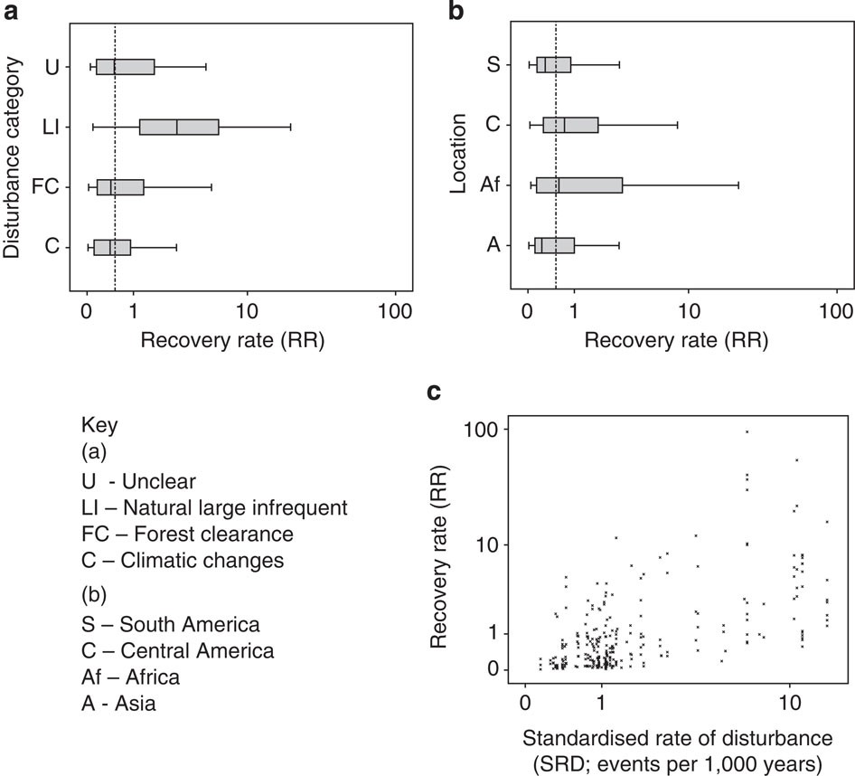
Three of the different factors we investigated for their potential effect on the forest recovery rate seemed to be of particular importance: geographical location, disturbance type and frequency of disturbance events. Of the four key tropical regions, Central American forests recovered the fastest and those in Asia the slowest (Figs. 2 & 3).  This is concerning, given that forests in Southeast Asia are currently experiencing some of the greatest rates of deforestation of all tropical regions, primarily due to the economic profitability of oil palm agriculture (check out mongabay for details).

Tropical forest recovery
Fig. 2  Map of tropical forest distribution, the location of studies and relative recovery rates across regions.

The most common form of disturbance, and one from which forest regrowth happened relatively slowly, was anthropogenic impact, i.e. via logging, burning and/or for agriculture (Fig. 3).  The slowest rates of recovery occurred after climatic disturbances and the fastest after large infrequent events, e.g. landslides, hurricanes and natural fire.  This latter result is somewhat intuitive given that these perturbations are a natural part of all ecosystems, leading to the evolution of a dynamic response in the native plant communities.  

Figure 3
Fig. 3  Composite figure showing how the recovery rate varies with different variables.

Insights into resilience

When we looked at the standardised rate of disturbance events (SRD), i.e. the number of disturbance events per 1,000 years, we found that the greater the frequency events occurred in the past, the more quickly the forest responded to each subsequent disturbance.  This runs counter to contemporary theories on resilience that describe slowing rates and diminishing ability to recover with each subsequent perturbation (e.g. Veraart et al., 2012).  Our results suggest that over ecologically meaningful timescales, i.e. over the life-span of entire forest communities rather than single trees, increased exposure results in adaptation to that disturbance over time, leading to a greater ability to recover quickly from the perturbation.

What does this all mean for tropical forests?

From looking back into the past, it seems that tropical forests can take a long time to recover from disturbances, and that different regions may require different management regimes to encourage more complete reforestation after natural or anthropogenic events, such as fire.  Central American and African forests may bounce back from impacts more quickly than the other regions, with disturbances such as tropical hurricanes and climatic fluctuations being a more common component of these ecosystems than in the other tropical regions.  However, all of the forests we looked at demonstrated a greater vulnerability to anthropogenic impacts and climatic changes than large infrequent disturbances: the two major forms of disturbance occurring today and at levels that far exceed those experienced over the past 20,000 years – reasons for caution.

Sustainable management

Identifying and understanding the different ecological requirements of forests across the different geographical regions, and of the forest-types within those regions, is vital for developing more sustainable landscape management plans.  With increasing international concern over deforestation rates, the associated loss of biodiversity and elevated carbon dioxide emissions, the conservation and restoration of tropical forests is becoming more politically and economically feasible.  Indonesia, for example, has introduced ‘ecosystem restoration concessions’ in the last decade, providing a legal means for forest protection from the further expansion of industrial agriculture.  And the potential of Reducing Emissions from Deforestation and Forest Degradation (now REDD+) to save the World’s forests continues to generate international debate. Of importance to all of these programmes and initiatives, is the suggestion from our study that forests take time to recover, and if we give them that time, they will persist, and continue to provide their faunal inhabitants, including us, the greatest collection of biological riches on Earth.

A half thought out critique

Inspired by a recent post by Joern Fischer I have decided to share one of my (many) half baked ideas. It’s based on a paper I read recently that I have a few issues with and want to work up into a letter to the editor, so please see all this as a work in progress and if you want to co-author it with me feel free, because that way I’m less likely to get a bad rep.So to the paper.Liu_coverIt’s this one by Liu et al in Global Ecology and Biogeography on how climate and age determine biomass in global mature forests.It sounded right up my street.I like forests.I like carbon. So I gave it a look.In the paper Liu et al aim to:

  • Investigate the relationship between aboveground biomass and climatic conditions and stand age in mature forests across the globe.
  •  Identify an age threshold at which forests should be considered ‘mature.’

The first question is interesting because people have done similar things with secondary forests in the past but I’m not sure I’ve ever seen this done looking at stand age in mature forests as a factor affecting biomass.The second I’m not a big fan of, but I will come to why later in the post.So Liu et al carry out a few analyses looking at the effects of mean annual temperature, mean annual rainfall, and stand age on biomass. However, the graphs of the analysis looks like this:Liu_fig_1 Liu_fig_2The figures had me worried and on closer inspection my suspicions were confirmed. They considered each explanatory variable independently in separate models. This is bad statistics but also doesn’t take account of the fact that previous studies have suggested that age, precipitation and temperature may interact to determine carbon accumulation rates. In addition the paper fails to account for spatial autocorrelation or differences between datasets that may be purely because of different methods used in their collection, rendering the results they present as questionable.To their credit Liu et al provide the data they used as supplementary materials so I thought I’d have a play with it to try and fix some of their errors.First I created a distance matrix and used that to look at spatial autocorrelation in biomass – surprise, surprise there were signs of spatial autocorrelation.I built a model that accounted for this and used a random effect to distinguish between each of the different datasets used in the study to account for between study error. I then did some model averaging so that all possible combinations of precipitation, temperature and age were included. I’ve put all of the code on github so feel free to look there and comment if you have any suggestions about the technical aspects of what I was up to.To cut a long story short the results suggest that all the variables considered by Liu et al are important, with one model that included all of them, as well as an interaction between temperature and age coming out as by far and away the best model.Age_tempTemp_age

Precipitation
Comparison of coefficients of our model compared to that of Liu et al. In each case the dotted black line represent’s Liu et al’s models and the coloured lines our models. Predictions were only made for interactions where there was sufficient data for both variables to allow this.


This model was much better than those of Liu et al (Table 1) – suggesting their approach was overly simplistic, as well as being statistically flawed. So, the models I developed explained much more variability than the equivalent ones in the Liu et al paper and changes the spin they put on their results.

Table 1 – Comparison of my top model and the models of Liu. AICc indicates relative parsimony of the model.

Model AICc AICc delta R squared
My model 623.98 0 0.29
Liu – Precipitation only 678.51 54.53 0.11
Liu – Temperature only 698.88 74.90 0.08
Liu – Age only 733.94 109.96 0.02


This model has an R squared 0.28, which is very good given the scale of the analysis but also suggests that there is quite a lot going on that we aren’t capturing in this model.  Part of this is probably because of the noise inherently added by using data collected in different ways.  In what I think is the best study of it’s type to date suggests that biomass in mature forests is only weakly related to commonly used climate metrics like mean temperature and mean precipitation. Instead, James Stegen and colleagues suggest that total biomass is well predicted by the biomass of the largest individual tree and that this is constrained by water deficit.

Now I to the second aim of Liu et al: to define a threshold age for mature forest.

This I have a big problem with. Even mature forests subject to relatively similar climatic conditions can vary massively in biomass and the reasons for this are not completely clear. Given this it is unwise to try to define a global threshold. It would be a much better idea to use chronosequence studies or long-term monitoring to try to discern dynamics at a landscape scale and build upon that to determine when forest should be classed as mature (and I’m only partly saying that because that’s what we did with secondary forest data…). I also have fears about defining ‘mature forest’ only using the biomass of these forests, and would be interested in seeing how biodiversity varies along with age in these old growth forests. Given that secondary forest carbon can get close to recovery quite quickly while biodiversity lags behind similar relationships may be seen for old growth forest. Any policy definition of what mature forest is could potentially have big implications for global biodiversity, so it important we get it right.

So those are my ideas. Critique them or add to them as you wish. And as I said, all code is available on github along with the data from the paper. I’m serious about writing a response, but like I said it needs more work so if you want to join me drop me a message below or in an email.

How long does tropical forest take to recover from agricultural clearance?

Secondaryforest4
Intermediate secondary forest in Paragominas, Para, Brazil – Photo credit to the fantastic Ricardo Solar, you can see more of his pics here

Today our work on the recovery of secondary tropical forests got published in Royal Society Proceedings B. I’m really chuffed with this piece of work and in this blog I’m going to summarise what we found out and why I think it’s important. If you want to read the paper you can get it here.

Large areas of tropical forest have been cleared for agriculture over the last 100 years.

Why does this matter? Well it matters because these forests are vital for the unique biodiversity in the tropics but also because humans can benefit from them remaining intact.

Their loss causes extinction, release of carbon into the atmosphere – worsening climate change, and changes the ecosystem services we get from these forests.

Because of the importance of these forests their restoration is seen as a priority by some. There are valiant attempts to restore tropical forests in Brazil and various Central American countries. In addition there are also international initiatives that aim to encourage the restoration of carbon and biodiversity (E.g. CBD & REDD+). These are great and ambitious aims but, until now, we didn’t really know how long these recoveries took, or whether recovery was different for different disturbance and forest types.

To solve all this we collected the biggest dataset yet compiled on recovery of aboveground, belowground and soil carbon as well as plant species richness and community composition following agricultural clearance. All this data came from previous studies.

Carbon_pools_colour

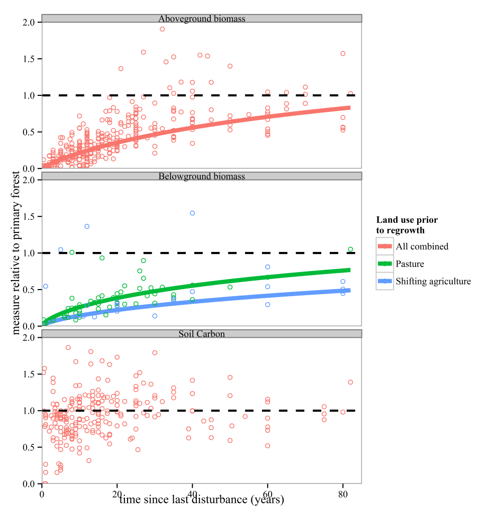
We found that after about 80 years aboveground carbon storage was around 85% of that found in undisturbed forests, while belowground carbon storage seemed to recover more slowly. Soil carbon showed no relationship with time since clearance.

Richness_colour

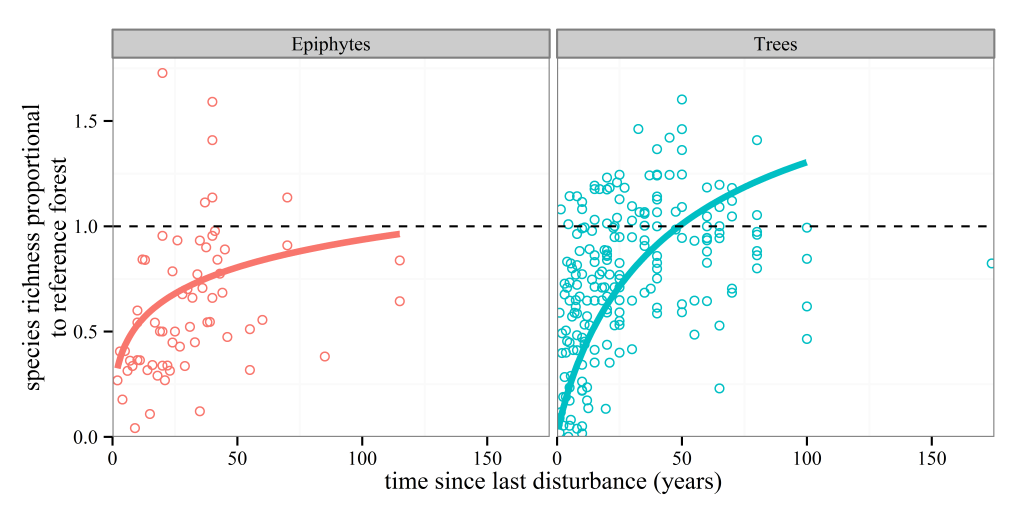
In terms of biodiversity both tree and epiphyte species richness seemed to increase over time, with tree richness recovering after around 50 years since disturbance but epiphytes took around 100 years.

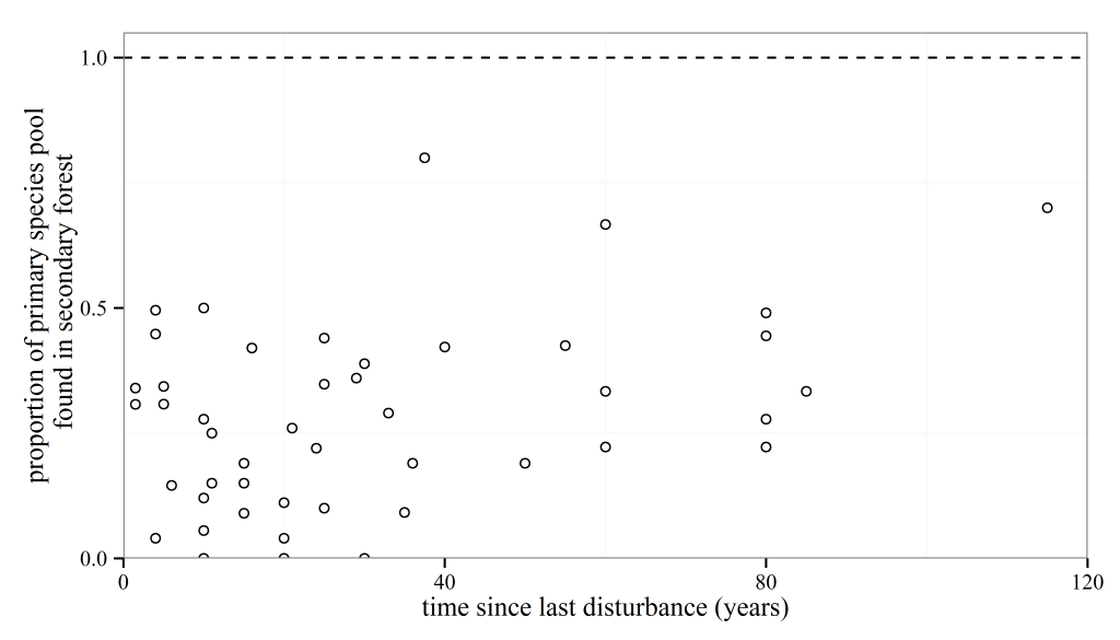
Prop_sp

However, when we looked at species that are found in the undisturbed forests, relatively few of them are found in the recovering forests. They didn’t seem to accumulate over time either. Given that these species are likely to be more prone to extinction it is worrying that they don’t seem to be doing very well in secondary forests.

We think that carbon recovers relatively well following abandonment of land since there tends to be a rapid influx of woody species. However, we also think that complete recovery of carbon is likely to take more than a century since this is likely to be dependent upon large, slow-growing trees.

Differences between tree species richness recovery and that of epiphytes is likely to be because tree seeds are more easily transported between forests than those of epiphytes. Also epiphytes seem to be found more on big trees, and there don’t tend to be many of these in secondary forests.

The lack of recovery of species found in undisturbed forests is perhaps the most disturbing thing that we found. We think that to improve this situation there may be a need for management of these forests by planting trees and helping to increase dispersal of seeds throughout the non-forest areas.

Disturbed forests like this are not worthless.
Regrowing forests like this are vital if we wish to conserve biodiversity in our human dominated world. Photo credit again to Ricardo Solar

There’s been lots of great work recently on the value of disturbed forests. We hope our work goes into a bit more detail where the soon-to-be-classic work of Luke Gibson etl al  left off which showed that primary forest has greater conservation value than any types of disturbed forest in the tropics. We agree with this, particularly for specialist species. However, most tropical forests are not primary forests and have been logged, cut down or burnt at some point in recent history. Because of this we think that older secondary forests need to be recognised as important for conservation and carbon storage and their clearance should be avoided. These forests are not worthless.

Experiments in fragmentation

Sites used by Biological Dynamics of Forest Fragments Project in Brazil

This is not really a proper post. It’s just here to highlight the great news article by Nature on experiments in tropical forest fragmentation. It backs up what I was saying in my article on the effects of logging on tropical biodiversity and talks a bit more about what the SAFE project is doing in Borneo in testing the effects of oil palm plantations and logging on forest structure and biodiversity. We need more of this kind of work and I’m really interested to see the first results from SAFE.

What traits drive response of birds to tropical land-use change?

Could fruit eating species such as the black-mandibled Toucan be disproportionately affected by land-use change?
Could fruit eating species like the black-mandibled Toucan be disproportionately affected by land-use change? (Photo credit to Ettore Bacocchi on flickr)

Everyone pretty much knows about the crisis of biodiversity loss facing the tropics.

In case you missed it tropical forests are being rapidly cleared, which human population increases and along with consumption. All this has lead to large losses of biodiversity in the tropics.

So far, so boring.

However, up until recently we didn’t have much of an idea how the characteristics of species in the tropics influenced their response to land-use change.

‘Why would we want to know that?’ – I hear you ask. Well if you’ve seen my blog before you will know that traits are  a good way of linking biodiversity change to changes in ecosystem function and services. This is the first step to working out the consequences of the massive changes in biodiversity we have seen over the last century. Simply put – we need to know this stuff.

Given what I think, it was great to find out at the recent BES 2012 annual meeting in Birmingham about a paper looking at how bird species with different traits respond to land-use change in the tropics.

Tim Newbold, a postdoc at the World Conservation Monitoring Centre in Cambridge, and colleagues compiled an impressive dataset of  >4500 records of >1300 bird species from 23 studies of  land-use change in the tropics. They then used data on habitat preferences, migratory status, diet, generation length and body size to determine how differences in these traits related to birds’ response to land-use change.

They found that long-lived, non-migratory, primarily frugiverous or insectivorous forest specialists were likely to be less abundant and less likely to occur in intensively used habitats.

Probabilities of presence and abundance relative to primary forest based on dietary preferences of tropical bird species

Of these characteristics diet preference is perhaps the most easy to link to changes in ecosystem function and services.

The loss of insect eating species may impact the control of pest species with potentially negative consequences for tropical agriculture. However, this assumption depends heavily on pest species abundances not reducing in line with bird declines. It is also entirely possible that if pest species also reduce in abundance forest loss will lead to little change in crop damage.

The reduction in fruit eating bird species may have consequences for forest regeneration and maintainance of plant diversity. Many secondary forests that are isolated from primary forest have been shown to lack large seeded tree species. Any reduction in the abundance of fruit eating birds suggests another barrier preventing the recovery of plant species communities in secondary forests.

I really liked this paper. It shows the value of large datasets for making generalisations and the results are potentially important for investigating change in ecosystem function and services in tropical forest ecosystems. The good news is it looks like there is a lot more of this type of work on the way with the PREDICTS project aiming to do take a similar approach to many questions related to land-use change. I’m excited to see what they come up with next, provided they don’t scoop me in the process…

Is secondary tropical forest of secondary importance?

Secondary cloud forest in Ecuador. Credit to Flickr user Peter Howe.

Everyone knows about the deforestation crisis that is going on. Most of this has taken place in the tropics and the majority of it has been as a result of agricultural expansion. However, less is made of the large growth of secondary tropical forest on abandoned pastures and agricultural land. In Central America in particular secondary succession has lead to increases in forest area, largely as a result of socio-economic changes and urbanisation. These secondary forests occupy large areas, but are obviously not equivalent to relatively undisturbed primary forests.

Plenty of research has been done comparing primary and secondary forest in the tropics. Luke Gibson and colleagues gave the most comprehensive overview of the differences between secondary and primary tropical forests in their recent Nature paper. In their meta-analysis they showed that secondary forests generally had lower biodiversity value, but also that they were more valuable than most other types of degraded forest.

However, this paper also oversimplified the value of tropical secondary forests.

It is widely known that secondary forests change dramatically with increasing age, and that older secondary forests are generally of greater conservation value. Firstly, secondary forests accumulate species richness of animal taxa reasonably quickly following abandonment, while plant species richness are likely to take a bit longer.

Change in species richness with time since last disturbance of secondary forest for bird and ant species. Adapted from Dunn et al 2004.

However, species richness is a rubbish measure of conservation value. It tells you nothing about the identity of the species present and therefore isn’t very useful. It can be higher in slightly disturbed forests than primary forests as a result of an influx of generalist species and a modest loss of forest specialists. So in the long run (>100 years) species richness in secondary forests should start to decrease back to levels similar to those found in primary forest.

Secondly,  the proportion of forest specialist species increases with age of secondary forest, again with vertebrate species colonising most quickly and plants logging behind. These differences are likely to be due to plants relatively limited dispersal ability.

Accumulation of old growth species in secondary tropical forests with increasing age, adapted from Chazdon et al 2009.

However, only about 50% of forest specialist plant species are present in the oldest tropical secondary forests we have records for. This poses the interesting questions about how long these communities take to recover, and whether they will ever reach similarity to primary forests.

Finally, secondary forest vertebrate communities may converge with those of primary forests after about 150 years. I have a few problems with the paper this analysis is taken from (presented blow), but at present it seems to be the best we have. I would actually argue that it suggests a relatively weak relationship between forest age and similarity, since the relationship largely depends on a few outliers amongst older forests. To get a better picture of what is going on we really need analysis which uses more secondary forests over 50 years old. This is a problem though, since most secondary forest is relatively young and it is difficult to age forest which is older than a couple of human generations.

Sorensen similarity change in vertebrate communities with increasing time since disturbance. Adapted from Dent et al 2009.

Despite the potential value of older secondary tropical forest, there is very little of it about. Much secondary forest is repeatedly cut as part of shifting agriculture and thus never develops communities characteristic of primary forest. In this way, the analysis of Gibson et al was probably correct, in that  most secondary forest is of lower value for conservation than primary forest.

However, if secondary forest is spared from conversion then it may be of great value in aiding the conservation of globally endangered species and carbon stocks in the face of expanding agriculture. Currently the greatest potential for this is likely to be in montane areas where the steep slopes make it difficult to access potential fields. However, outside of dedicated restoration projects, encouraging secondary growth will be difficult.

This is a subject I will return to in the coming weeks and months since I am currently working on a project investigating some of these issues. Meanwhile if you have anything to say,  leave a comment below.

Update: I have just gathered together the code I used to make the graphs in these posts and since I haven’t had time to write a blog post this week, I thought I’d post this instead.

Code for the Dunn et al graph:

#load in Data from Dunn et al paper
Dunn<-structure(list(Age = c(1.002, 0.9979, 0.9939, 0.9938, 5.0048, 10.9567, 10.9973, 14.0228, 17.1238, 20.9715, 51.3436, 41.19, 1.0014, 0.9973, 0.9935, 0.9931, 0.9965, 2.0012, 1.9931, 1.9997, 3.0166, 6.0685, 10.9948, 6.0292, 6.0752, 9.0246, 18.1524, 21.1961, 26.3481, 37.611, 41.4627), Species.richness = c(89.1859, 68.5023, 49.7654, 44.4118, 46.0596, 73.4128, 76.5756, 84.3176, 103.0184, 90.3269, 93.8115, 127.434, 63.148, 40.0309, 31.2711, 12.2903, 6.936, 63.02, 46.9599, 29.6817, 98.4726, 72.062, 66.1117, 105.6449, 121.2176, 149.8593, 118.0951, 80.5911, 84.9311, 115.0402, 98.718), Taxa = structure(c(1L, 1L, 1L, 1L, 1L, 1L, 1L, 1L, 1L, 1L, 1L, 1L, 2L, 2L, 2L, 2L, 2L, 2L, 2L, 2L, 2L, 2L, 2L, 2L, 2L, 2L, 2L, 2L, 2L, 2L, 2L), .Label = c("Ants","Birds"),class = "factor")), .Names = c("Age","Species.richness", "Taxa"), class = "data.frame", row.names = c(NA,-31L))                                                                                                                                                                                                                                                                                                                                                                   

#load packages needed
library(ggplot2)

#graph relationship
a<-ggplot(Dunn,aes(x=Age,y=Species.richness/100,alpha=0.5,colour=Taxa))
b<-a+geom_point(size=3,shape=16)+scale_area(c(1,3))+theme_bw()
c<-b+theme(legend.position = "none")+theme(panel.grid.major = element_line(colour =NA))+theme(axis.title.x = element_text(size = 12, colour = 'black'))+theme(axis.title.y = element_text(angle=90,size = 12, colour = 'black'))
d<-c+ylab ('Species richness \nrelative to primary forest')+xlab ('Age of secondary forest (Years)')
d+xlim(0,60)+ylim(0,1.6)+geom_hline(y=1,lty=2)+stat_smooth(se=F,method="lm",formula = y ~ x+I(x^2),size=1)+coord_cartesian(xlim =c(0,55), ylim =c(0,1.6), wise = NULL)+facet_wrap(~Taxa)

#save plot
ggsave("Dunn et al 2009.png",height=3,width=6,dpi=1200)

Created by Pretty R at inside-R.org

Code for the Chazdon et al 2009 graph:

#load in data
chaz<-structure(list(Sqrt_age = c(10.0405, 6.3648, 5.5131, 5.5105, 5.0395, 4.2022, 3.9136, 3.6978, 3.1653, 2.9973, 2.8463, 2.2557, 1.7412, 5.2755, 3.8921, 2.9493, 2.2355, 2.2341, 2.2147, 0.9659, 5.0391, 3.6583, 3.2024, 2.96, 5.946, 5.0492, 4.1573, 3.6404,  3.1997, 3.4873, 2.9569, 2.8628, 2.7869, 2.257, 3.6512, 1.7506, 2.2671, 5.3014, 4.2211, 4.5083, 3.9005, 3.201, 3.1851, 2.2463, 2.0025, 2.0163, 0.9811, 2.2387, 1.9766, 4.4682, 3.287, 3.8925, 3.8793, 3.8959, 4.9149, 4.6122, 3.3359, 4.0257, 4.9985, 5.4059,  5.7681, 5.002, 6.023, 7.117, 9.0111), Proportion = c(0.8328, 0.8632, 0.8401, 0.7619, 0.7617, 0.7117, 0.713, 0.6218, 0.6002, 0.5789, 0.6017, 0.6599, 0.721, 0.5495, 0.5308, 0.502, 0.5104, 0.4705, 0.3495, 0.2594, 0.7504, 0.8013, 0.7997, 0.821, 0.611,  0.5979, 0.7302, 0.7215, 0.7185, 0.6886, 0.7285, 0.6401, 0.6415, 0.6998, 0.5918, 0.5501, 0.5503, 0.4215, 0.3713, 0.3273, 0.3271, 0.3084, 0.2871, 0.3822, 0.3594, 0.3181, 0.258, 0.1558, 0.043, 0.041, 0.1546, 0.0921, 0.1491, 0.1904, 0.2192, 0.2589, 0.2529, 0.4325, 0.4456, 0.3531, 0.2906, 0.0906, 0.191, 0.1912, 0.4922), Type = structure(c(1L, 1L, 1L, 1L, 1L, 1L, 1L, 1L, 1L, 1L, 1L, 1L, 1L, 1L, 1L, 1L, 1L, 1L, 1L, 1L, 2L, 2L, 2L, 2L, 2L, 2L, 2L, 2L, 2L, 2L, 2L, 2L, 2L, 2L, 2L, 2L, 2L, 2L, 2L, 2L, 2L, 2L, 2L, 2L, 2L, 2L, 2L, 2L, 3L, 3L, 3L, 3L, 3L, 3L, 3L, 3L, 3L, 3L, 3L, 3L, 3L, 3L, 3L, 3L, 3L), .Label = c("Flying animals", "Non-flying animals", "Trees"), class = "factor")), .Names = c("Sqrt_age", "Proportion", "Type"), class = "data.frame", row.names = c(NA, -65L))

#load ggplot2
library(ggplot2)

#graph relationship
a<-ggplot(chaz,aes(x=Sqrt_age^2,y=Proportion,alpha=0.5,colour=factor(Type)))
b<-a+geom_point(size=2)+stat_smooth(method="glm",formula = y ~ x,se=F,size=1)+scale_area()+scale_colour_manual(values=c("red","blue","orange"))
c<-b+theme_bw()+facet_wrap(~Type)
d<-c+theme(legend.position = "none")+theme(panel.grid.major = element_line(colour =NA))+theme(axis.title.x = element_text(size = 20, colour = 'black'))+theme(axis.title.y = element_text(angle=90,size = 20, colour = 'black'))
e<-d+ylab ('Proportion of \nold growth species')+xlab ('Age of secondary forest (Years)')
e+coord_cartesian(xlim=c(0,110),ylim=c(0,1))

#save plot
ggsave("Chazdon et al 2009 facet.png",height=3,width=6,dpi=1200)

Created by Pretty R at inside-R.org

Code for Dent et al 2009 graph:

#load in data
dent<-structure(list(Age = c(151.2753, 141.0416, 101.2877, 91.0569, 81.1214, 101.0649, 60.6883, 90.067, 70.3094, 65.2109, 40.6187, 23.5788, 8.3336, 9.371, 30.9226, 26.8362, 8.4707, 10.8033, 4.8007, 17.7511, 8.1344, 30.5806, 25.9007, 25.8831, 9.5432, 14.1966, 18.5549, 6.6113, 6.3277, 3.6179, 5.6787, 12.6911, 15.6025, 17.6164, 35.5596, 20.8186, 17.1589, 8.4203, 13.6423, 10.2735, 13.6131, 5.8801, 10.6768, 27.9142, 26.7288, 35.7948, 5.6885, 8.2841, 15.4354,11.6134, 25.3636, 30.4658, 26.3691, 27.9504, 24.2643, 5.4647, 5.2966, 5.2819, 8.9196, 13.1625, 14.1797, 15.9203, 8.8961, 5.5332, 5.4643, 4.6837, 25.068, 25.3471, 25.1892, 32.5845, 10.2331, 16.7896, 16.7617, 20.2606, 5.2405, 2.1346, 4.3152, 4.1426, 10.0807, 14.9214, 1.0177, 0.8349, 4.0356, 0.7206, 3.8641, 4.9122, 7.8045, 14.8184, 35.0082, 9.7931, 13.7407), Similarity = c(1.0252, 1.0216, 1.0161, 1.0147, 1.0156, 0.8468, 0.8122, 0.4842, 0.3501, 0.5844, 0.8852, 0.9285, 1.0034, 0.9032, 0.846, 0.8498, 0.8853, 0.8812, 0.8725, 0.8309, 0.8518, 0.8081, 0.8052, 0.7919, 0.8119, 0.7947, 0.7753, 0.8048, 0.8115, 0.7509, 0.7623, 0.761, 0.7526, 0.7283, 0.7052, 0.7187, 0.7138, 0.736, 0.7066, 0.7006, 0.6843, 0.6933, 0.6739, 0.6696, 0.6572, 0.6617, 0.6587, 0.6322, 0.6255, 0.6082, 0.6191, 0.6098, 0.6059, 0.5859, 0.561, 0.5996, 0.5829, 0.5718, 0.56,  0.5638, 0.5596, 0.5497, 0.5422, 0.5406, 0.4882, 0.4502, 0.5053, 0.4954, 0.4865, 0.4429, 0.4476, 0.4329, 0.4118, 0.4056, 0.4291, 0.4009, 0.3921, 0.3721, 0.3317, 0.3458, 0.3294, 0.3014, 0.2908, 0.2146, 0.1604, 0.1795, 0.1565, 0.1564, 0.1747, 0.0019, 0.00356), Similarity2 = c(0.9992, 0.9956, 0.9901, 0.9887, 0.9896, 0.8208, 0.7862, 0.4582, 0.3241, 0.5584, 0.8592, 0.9025, 0.9774, 0.8772, 0.82, 0.8238, 0.8593, 0.8552, 0.8465, 0.8049, 0.8258, 0.7821, 0.7792, 0.7659, 0.7859, 0.7687, 0.7493, 0.7788, 0.7855, 0.7249, 0.7363, 0.735, 0.7266, 0.7023, 0.6792, 0.6927, 0.6878, 0.71, 0.6806, 0.6746, 0.6583, 0.6673, 0.6479, 0.6436, 0.6312, 0.6357, 0.6327, 0.6062, 0.5995, 0.5822, 0.5931, 0.5838, 0.5799, 0.5599,  0.535, 0.5736, 0.5569, 0.5458, 0.534, 0.5378, 0.5336, 0.5237,  0.5162, 0.5146, 0.4622, 0.4242, 0.4793, 0.4694, 0.4605, 0.4169, 0.4216, 0.4069, 0.3858, 0.3796, 0.4031, 0.3749, 0.3661, 0.3461, 0.3057, 0.3198, 0.3034, 0.2754, 0.2648, 0.1886, 0.1344, 0.1535, 0.1305, 0.1304, 0.1487, 0.0019, 0.00356)), .Names = c("Age", "Similarity", "Similarity2"), class = "data.frame", row.names = c(NA, -91L))

#load ggplot2
library(ggplot2)

#graph relationship
a<-ggplot(dent,aes(x=Age,y=Similarity2,alpha=0.5))
b<-a+geom_point(size=3,shape=16,colour="red")
c<-b+scale_area(c(1,3))+theme_bw()
d<-c+theme(legend.position = "none")+theme(panel.grid.major = element_line(colour =NA))+theme(axis.title.x = element_text(size = 12, colour = 'black'))+theme(axis.title.y = element_text(angle=90,size = 12, colour = 'black'))
e<-d+ylab ('Sorensen similarity')+xlab ('Age of secondary forest (Years)')
e+xlim(0,160)+ylim(0,1)+geom_hline(y=1,lty=2)+stat_smooth(se=F,method="lm",formula = y ~ x+I(x^2),size=1)+coord_cartesian(xlim =c(0,151), ylim =c(0,1.1), wise = NULL)

#save plot
ggsave("Dent et al 2009.png",height=3,width=6,dpi=1200)

Created by Pretty R at inside-R.org